
The Solitary Wave Theory, have soliton-like solutions of nonlinear evolution equations describing wave process in dispersive and dissipation media [6]. A sketch of these types of waves is shown below
2.1 Soliton
A soliton [14] is a solitary wave which asymptotically preserves its shape and velocity upon nonlinear interaction with other solitary waves. Soliton has following properties
- They are of permanent form.
- They are localized within a region.
- They can interact with other solitons and emerge from the collision unchanged, except for a phase shift.
- Soliton is caused by a delicate balance between nonlinear and dispersive effects.
2.2 Travelling Wave
Travelling wave [14] can be defined as a wave in which the medium is travelling in the direction of propagation of wave. Travelling waves arises in the study of nonlinear differential equations where waves are represented by the form
u(x,t) = f(x-ct)
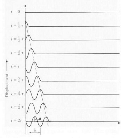 Figure (2.2)-Travelling Waves
and c is the speed of wave propagation. For c < 0 , the wave moves in the positive direction whereas the wave moves in the negative x direction for c < 0.
2.2.1 Types of Travelling Wave Solutions
Travelling wave solutions are of many types and they are of particular importance in solitary wave theory. Here we are going to describe six different types of travelling wave solutions with their figures.
Definition 1.1. Solitary waves [14] are localized travelling waves with constant speeds and shapes, asymptotically zero at large distance solutions. Solitons are special kind of solitary waves. The soliton solution is a spatially localized solution, hence
![]()
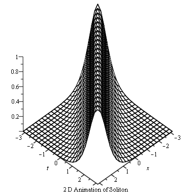
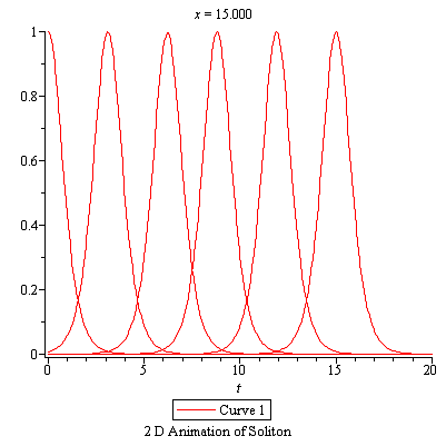
The KdV equation is a pioneer model for analytic bell-shaped sech² solitary wave solutions.
Definition 1.2. Kink waves [14] are travelling waves which rise or descend from one asymptotic state to another. The Kink solution approaches a constant at infinity. The standard dissipative burgers equation
![]()
is a well-known equation that gives kink solutions where v is the viscosity coefficient.
The graphical representation of Kink wave is
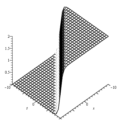
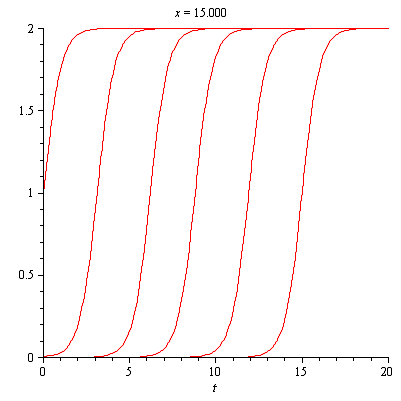
Figure (2.4) – General Representation of Kink Waves Figure (2.4) – 2D-Animation
Definition 2.19. Periodic waves [14] are travelling wave that are periodic such as cos(x-t) . The standard wave equation ![]() gives periodic solutions. Graphical representation is given below
gives periodic solutions. Graphical representation is given below
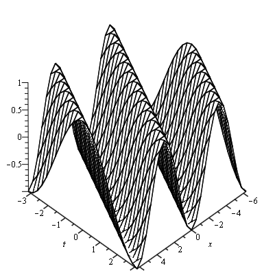
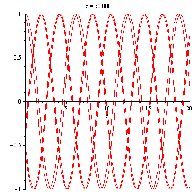
Figure (2.5) – General Representation of Periodic Waves Figure (2.5) – 2D Animation
Definition 2.20. Peakons [14] are the solitary wave solutions. In this case the travelling solutions are the smooth except for a peak at a corner of its crest. The peakons are solutions retaining their shape and speed after interacting. Peakons were investigated and classified as a periodic peakons and peakons with exponential decay. Some graphical representations of peakons are given below
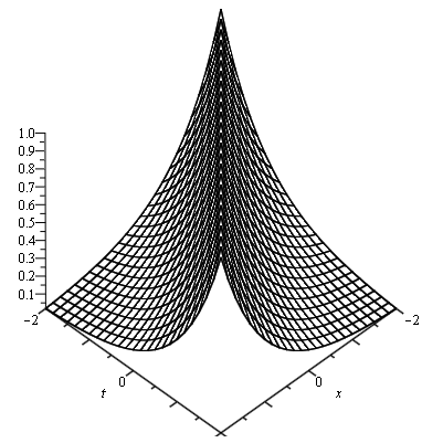
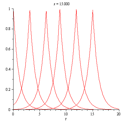
Figure (2.6) – General Representation of Peakons Figure (2.6) – 2D Animation
Definition 2.21. Cuspons [14] are other form of solitons where solution exhibit cusps at their crests. Unlike Peakons where the derivative at the peak differs only by a sign, the derivative at the jump of a Cuspons diverges. It is important to note that the Soliton solution u(x,t), along with its derivatives tends to zero as ![]() Cuspons were investigated and classified as periodic Cuspons and Cuspons with exponential decay.
Cuspons were investigated and classified as periodic Cuspons and Cuspons with exponential decay.
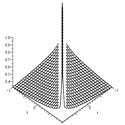
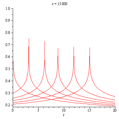
Figure (2.7)-General Representation of Cuspons
Definition 2.22. It is new class of Soliton with compact spatial support such that each compacton is a Soliton confined to a finite core. Compactons [14] has some properties and we can describe it in one of the following ways:
- Compactons are Solitons with finite wavelength.
- Compactons are solitary waves with compact support.
- Compactons are Solitons free of exponential tail.
- Compactons are Solitons characterized by the absence of infinite wings.
- Compactons are robust Soliton-like solutions.
Graphical representation is given below
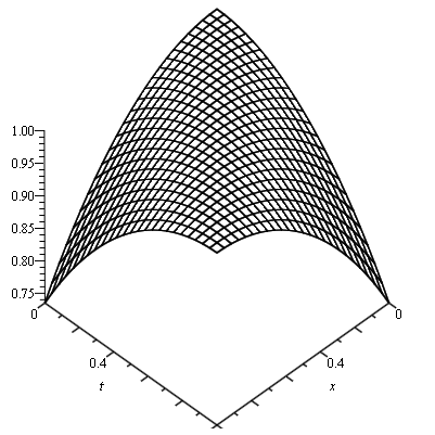
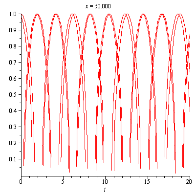
Figure (2.8) – General Representation of Compactons Figure (2.8) – 2D Animation
2.2 Some Basic Definitions of Wavelets Theory
2.2.1 History
Wavelet analysis developed in the largely mathematical literature in the 1980’s and began to be used commonly in geophysics in the 1990’s. Wavelets can be used in signal analysis, image processing and data compression. They are useful for sorting out scale information, while still maintaining some degree of time or space locality.
2.2.2 Wavelets
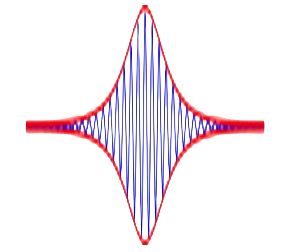
A wavelet [11, 16] is a wave-like oscillation that is localized in the sense that it grows from zero, reaches maximum amplitude, and then decreases back to zero amplitude again. It thus has a location where it maximizes, a characteristic oscillation period, and also a scale over which it amplifies and declines. The following figure represents Wavelets constitute a family of function constructed from dilaition
2.2.3 Types of Wavelets
According to Meyer (1993), two fundamental types of wavelets [16] can be considered,
- The Grossmann-Morlet time-scale wavelets
- The Gabor-Malvar time-frequency wavelets.
Time-scale wavelets are defined in reference to a “mother function” ψ(t) of some real variable t .The mother function can be used to generate a whole family of wavelets by translating and scaling the mother wavelet.
![]()
Here is the translation parameter and is the scaling parameter. Provided that ψ(t) is real-valued, this collection of wavelets can be used as an orthonormal basis. If we restrict the parameters and to discrete values as ![]() and n,k are positive integers, we have the following family of discrete wavelets
and n,k are positive integers, we have the following family of discrete wavelets
![]()
where ![]() forms an orthogonal basis.
forms an orthogonal basis.
2.2.4 Functions Approximation
A function f(t) define over [0, 1) may be expanded [46] as
![]()
where ![]() in which
in which ![]() denotes the inner product. If the infinite series in Eq. is truncated, then above Eq. can be written as
denotes the inner product. If the infinite series in Eq. is truncated, then above Eq. can be written as
![]() It can be written as
It can be written as
![]()
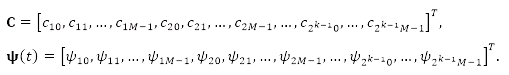
where C and ψ(t) are ![]() matrices given as
matrices given as
References
[1]S. Abbasbandy, Numerical solutions of the integral equations: Homotopy perturbation method and Adomian’s decomposition method, Appl. Math. Comput. 173(23) (2006), 493-500.
[2]Z. Avazzadeh, B. Shafiee and G. B. Loghmani, Fractional calculus for solving Abel’s integral equations using Chebyshev polynomials, Applied Mathematical Sciences, 5(45)(2011), 2207 – 2216
[3]Subhra Bhattacharya, Use of bernstein polynomials in numerical solutions of volterra integral equations: Applied Mathematical Sciences, 2(36)(2008), 1773 – 1787.
[4]Caputo, Michel, Linear model of dissipation whose Q is almost frequency independent-II. J. R. Astr. Soc. 13 (1967), 529–539.
[5]M.E. Fettis, On numerical Solution of Equations of the Abel type, Math. Comp. 18(1964), 491–496.
[6]J. Garza, P. Hall, F.H. Ruymagaart, A new method of solving noisy Abel-type equations, J. Math. Anal. Appl. 257 (2001), 403–419.
[7]P. Hall, R. Paige, F.H. Ruymagaart, Using wavelet methods to solve noisy Abel-type equations with discontinuous inputs, J. Multivariate. Anal. 86 (2003), 72–96.
[8]Li Huang, Yong Huang, Xian-Fang Li, Approximate Solution of Abel Integral Equation, Computers and Mathematics with Applications 56 (2008), 1748–1757.
[9]A. Hwang and Y. P. Shih, Solution of integral equations via Laguerre polynomials, Comput. Electr. Engrg. 9 (1982), 123–129
[10]D.A. Murio, D.G. Hinestroza, C.W. Mejia, New stable numerical inversion of Abel’s integral equation, Comput. Math. Appl. 11(1992), 3–11.
[11]D.E. Newland, An Introduction to random vibrations, spectral and wavelet analysis, longman scientific and technical, New York, (1993).
[12]R.Piessens, Computing integral transforms and solving integral equations using Chebyshev polynomial approximations, J. Comput. Appl. Math. 121 (2000),113–124.
[13]R.Piessens, P. Verbaeten, Numerical solution of the Abel integral equation, BIT 13 (1973), 451–457.
[14]A.M. Wazwaz, Partial Differential Equations and Solitary Waves Theory, HEP and Springer, Beijing and Berlin, (2009).
[15]J. Y. Xiao, L. H. Wen, D. Zhang, Solving second kind integral equations by periodic wavelet Galerkin method, Appl. Math. Comput.175(2006), 508-518.
[16] S.A.Yousefi, Numerical solution of Abel’s integral equation by using Legendre wavelets, Applied Mathematics and Computation,175 (2006), 574-580.