
Fractional Calculus and Definitions of Integral Equations, we have focused on numerical and traveling wave solutions of linear and nonlinear integral and partial differential equations that describe a variety of physical phenomena. It is one of the important tasks in the study of partial differential equations to seek the exact solutions. In the past several decades both mathematicians and physicists have made many attempts in this field. Several methods are used to study the nonlinear differential equations.
1.1 Preliminary Definitions
We divided into two sections. First section contains some basic preliminaries of fractional calculus, second section is about some basic definitions of integral equations are given
1.2 Preliminaries of Fractional Calculus
1.1.1 History
Fractional calculus has its origin in the question of the extension of meaning. A well known example is the extension of meaning of real numbers to complex numbers, and another is the extension of meaning of factorials of integers to factorials of complex numbers. In generalized integration and differentiation the question of the extension of meaning is: Can the meaning of derivatives of integral order![]() be extended to have meaning where n is any number irrational, fractional or complex?
be extended to have meaning where n is any number irrational, fractional or complex?
Leibnitz invented the above notation. Perhaps, it was naive play with symbols that prompted L’Hôpital to ask Leibnitz about the possibility that n be a fraction. “What if n be ½?” asked L’Hôpital. Leibnitz in 1695 replied, “It will lead to a paradox.” But he added prophetically, “From this apparent paradox, one day useful consequences will be drawn.” In 1697, Leibnitz [4], referring to Wallis’s infinite product for , used the notation
![]() and stated that differential calculus might have been used to achieve the same result.
and stated that differential calculus might have been used to achieve the same result.
In 1819 the first mention of a derivative of arbitrary order appears in a text. The French mathematician S. F. Lacroix [2] published a 700 page text on differential and integral calculus in which he devoted less than two pages to this topic.
Summary of above discussion
In the letters to J. Wallis and J. Bernoulli (in 1697) Leibniz mentioned the possible approach to fractional-order differentiation in that sense, that for non-integer values of n the definition could be the following:
 Euler suggested using this relationship also for negative or non-integer (rational) values of n. Taking m=1 , n= ½ Euler obtained:

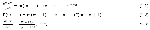
1.1.2 Fractional Derivative of a Basic Power Function
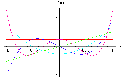
The half derivative (purple curve) of the function f(x) =x (blue curve) together with the first derivative (red curve). Let us assume that f(x) is a monomial of the form
![]()
The first derivative is as usual
![]() Repeating this gives the more general result that
Repeating this gives the more general result that
 Which after replacing the factorials with the Gamma function, leads us to
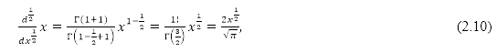
 For k=1 and α=1/2 , we obtain the half-derivative of the function x as
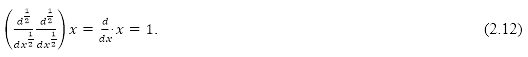
 Repeating this process yields
 Which is indeed the expected result of
 This extension of the above differential operator need not be constrained only to real powers. For example, the (1+i)th derivative of the (1+i)th derivative yields the 2nd derivative. Also notice that setting negative values for yields integrals.
For a general function f(x) and 0 < α < 1 , the complete fractional derivative is
![]()
For arbitrary α, since the gamma function is undefined for arguments whose real part is a negative integer, it is necessary to apply the fractional derivative after the integer derivative has been performed. For example,
![]()
1.1.3 Fractional Integrals
The classical form of fractional calculus is given by the Riemann–Liouville integral, essentially what has been described above. The theory for periodic functions, therefore including the ‘boundary condition’ of repeating after a period, is the Weyl integral. It is defined on Fourier series, and requires the constant Fourier coefficient to vanish (so, applies to functions on the unit circle integrating to 0).
Definition 1.1. The Riemann-Liouville fractional integral operator [6] of order ![]() of a function
of a function ![]() is defined as
is defined as
 properties of the operator
 ![]() we mention only the following:For
we mention only the following:For ![]() and
and ![]()

The Riemann-Liouville derivative has certain disadvantages when trying to model real-world phenomena with fractional differential equations.
1.1.4 Fractional Derivatives
Not like classical Newtonian derivatives, a fractional derivative is defined via a fractional integral.
Definition 1.2. The Riemann–Liouville fractional derivative [5] of order α for a function f is defined by
![]()
Note: the main disadvantage of Riemann–Liouville fractional derivative is that the fractional derivative of a constant is not zero. If f = C , then
![]()
Definition 1.3. The modified Riemann–Liouville [3] derivative is defined as
![]()
Definition 1.4. There is another option for computing fractional derivatives; the Caputo fractional derivative. It was introduced by M. Caputo [1] in 1967 in his celebrated paper. In contrast to the Riemann Liouville fractional derivative, when solving differential equations using Caputo’s definition, it is not necessary to define the fractional order initial conditions. Caputo’s definition is illustrated as follows; the fractional derivative of f(t) in the Caputo sense is defined as
![]() for
for ![]() Fractional derivative of any order
Fractional derivative of any order
Caputo
![]()
Riemann-Liouville

1.3 Introductory Concepts of Integral Equations
1.3.1 Integral Equations
Any functional equation in which the unknown function appears under the sign of integration is called an integral equation.
![]() where
where
- α(x)and β(x) are limits of integration,

- λ is a constant parameter
- k(x,t) is a function of two variables and
- The function u(x) is unknown and
- The functions f(x) real function.
1.3.2 Classifications of Integral Equations
Integral equations appear in many forms. Two distinct ways that depend on the limits of integration are used to characterize integral equations, namely:
Definition 1.5. If the limits of integration are fixed, the integral equation is called a Fredholm integral equation given in the form:
![]()
where a and b are constants.
Definition 1.6. If at least one limit is a variable, the equation is called a Volterra integral equation given in the form:
![]()
Moreover, two other distinct kinds, which depend on the appearance of the unknown function u(x), are defined as follows:
Definition 1.7 If the unknown function μ(x) appears only under the integral sign of Fredholm integral equation, the integral equation is called a first kind Fredholm integral equation.
![]()
Definition 1.8 If the unknown function μ(x) appears only under the integral sign of Volterra integral equation, the integral equation is called a first kind Volterra integral equation.
![]()
Definition 1.9. If the unknown function μ(x) appears both inside and outside the integral sign of Fredholm integral equation, the integral equation is called a second kind Fredholm integral equation
![]()
Definition 1.10. If the unknown function μ(x) appears both inside and outside the integral sign of Volterra integral equation, the integral equation is called a second kind Volterra integral equation
![]()
Definition 1.11. In all Fredholm integral equations presented above, if f(x) is identically zero, the resulting equation: is called homogeneous Fredholm integral equation
![]()
Definition 2.12. In all Volterra integral equations presented above, if f(x) is identically zero, the resulting equation: is called homogeneous Volterra integral equation
![]()
1.3.3 Integro-Differential Equation
It is interesting to point out that any equation that includes both integrals and derivatives of the unknown function μ(x) is called integro-differential equation.
Definition 1.13. The Fredholm integro-differential equation is of the form:
![]()
Definition 1.14. The Volterra integro-differential equation is in the form:
![]()
1.3.4 Linearity Concept
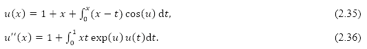
If the exponent of the unknown function μ(x) inside the integral sign is one, the integral equation or the integro-differential equation is called linear. If the unknown function μ(x) has exponent other than one, or if the equation contains nonlinear functions μ(x)of such as sinh(μ), cos(μ), ln(1+μ) the integral equation or the integro-differential equation is called nonlinear. To explain this concept, we consider the equations:
1.3.5 Homogeneity Concept
Integral equations and integro-differential equations of the second kind are classified as homogeneous or inhomogeneous, if the function f(x) in the second kind of Volterra or Fredholm integral equations or integro-differential equations is identically zero, the equation is called homogeneous. Otherwise it is called inhomogeneous. Notice that this property holds for equations of the second kind only. To clarify this concept we consider the following equations

1.3.6 Singular Integral Equations
Volterra integral equations of the first kind
![]()
or of the second kind
![]()
are called singular if:
- One of the limits of integration g(x), h(x) or both are infinite, or
- If the kernel k(x,t) becomes infinite at one or more points at the range of integration.

Definition 1.15. The Abel’s integral equations is given as
![]()
Definition 1.16. If α < n the kernel (and the integral) is called weakly singular then Eq. (3.24) is called weakly singular integral equation.
References
[1]. Caputo, Michel, Linear model of dissipation whose Q is almost frequency independent-II. J. R. Astr. Soc. 13 (1967), 529–539.
[2]. Mehdi Dalir and Majid Bashour, Applications of Fractional Calculus, Applied.
[3].G. Jumarie, Table of some basic fractional calculus formulae derived from a modified Riemann–Liouville derivative for non-differentiable functions, Appl. Math. Lett, 22 (2009), 378–385.
[4]. De-Gang Wang, Wen-Yan Song, Peng Shi and Hamid Reza Karimi, Approximate analytic and numerical solutions to Lane-Emden equation via fuzzy modeling method, mathematical problems in engineering,Article ID 259494, 15 pages, doi:10.1155/2012/259494,(2012).
[5]. M. Wazwaz, Partial Differential Equations and Solitary Waves Theory, HEP and Springer, Beijing and Berlin, (2009).
[6]. Li Zhu, Qibin Fan, Solving fractional nonlinear Fredholm integro-differential equations by the second kind Chebyshev wavelet, Commun Nonlinear Sci Numer Simulat 17 (2012), 2333–2341.