
Bessel Polynomial Method,we develop a new algorithm for solving linear and nonlinear integral equations using Galerkin weighted residual numerical method with Bessel polynomials [1]. Bessel polynomials is given as

3.8.1 Methodology
Definition 3.7. Consider the integral equation of the 1st kind is given as
![]()
where u(t) is the unknown function, to be determined, k(x,t) , the kernel, is a continuous or discontinuous and square integrable function, f(x) being the known function.
Now we use the technique of Galerkin method, [Lewis, 2], to find an approximate solution ![]() . For this, we assume that
. For this, we assume that
![]()
where ![]() are Bessel polynomials of degree defined in equation (5.546) and
are Bessel polynomials of degree defined in equation (5.546) and ![]() are unknown parameters, to be determined.
are unknown parameters, to be determined.
substituting (3.200) into (3.199),
we get,
![]()
Then the Galerkin equations are obtained by multiplying both sides of (3.201) by ![]() and then integrating with respect to x from a to b , we have
and then integrating with respect to x from a to b , we have
![]()
Since in each equation, there are two integrals. The inner integrand of the left side is a function of x, and t, and is integrated with respect to t from a to x. As a result the outer integrand becomes a function of x only and integration with respect x to from a to b yields a constant. Thus for each j=0,1,2,…,n we have a linear equation with n+1 unknowns ![]() , k=0,1,2,…,n.
, k=0,1,2,…,n.
Finally (3.202) represents the system of n+1 linear equations in n+1 unknowns, are given by
![]()
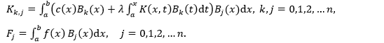
where
![]()
and
![]()
Now the unknown parameters ![]() are determined by solving the system of equations (3.203) and substituting these values of parameters in (3.200), we get the approximate solution
are determined by solving the system of equations (3.203) and substituting these values of parameters in (3.200), we get the approximate solution ![]() of the integral equation (3.199).
of the integral equation (3.199).
Definition 3.8. Consider the integral equation of the 2nd kind is
![]()
where u(t) is the unknown function, to be determined, k(x,t) , the kernel, is a continuous or discontinuous and square integrable function, f(x) and u(x) being the known function and λ is a constant. Proceeding as before
![]()
where
Now the unknown parameters ![]() are determined by solving the system of equations (3.205) and substituting these values of parameters in (3.197), we get the approximate solution
are determined by solving the system of equations (3.205) and substituting these values of parameters in (3.197), we get the approximate solution ![]() of the integral equation (3.204).
of the integral equation (3.204).
3.8.2 Applications of Bessel Polynomial Method
Example 3.34 Consider the linear Volterra Integral equation [2]
![]()
The exact solution of Eq. (3.206)
![]()
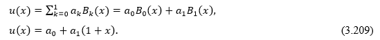
According to the proposed technique, consider the trail solution
![]()
Consider 1st order Bessel Polynomials, i.e. for n=1, we have Eq. (3.208) is
Substituting Eq. (3.209) into Eq. (3.206)
![]()
Now multiply Eq. (3.210) by ![]() j=0,1 and integrating both side from 0 to 1, we have
j=0,1 and integrating both side from 0 to 1, we have

the matrix form of Eq. (3.211) is

After solving we get ![]() and
and ![]() Consequently we have the approximate solution is
Consequently we have the approximate solution is
u(x) = -0.1333+1.7499x.
Table 3.28 Comparison of the Exact Solution and Approximate Solutions of Eq. (3.206) for n=1 using Bessel Polynomial Method


Fig 3.28 Comparison of Exact and Approximate Solutions of Eq. (3.206) for n=1.
Consider 2nd order Bessel Polynomials, i.e. for n=2, we have Eq. (3.208) is

Substituting Eq. (3.212) into Eq. (3.206)

Now multiply Eq. (3.213) by ![]() j=0,1,2 and integrating both side from 0 to 1, we have
j=0,1,2 and integrating both side from 0 to 1, we have

the matrix form of Eq. (3.214) is

After solving we get
![]()
Consequently we have the exact solution is
u(x) = x+ x².
Table 3.29 Comparison of the Exact Solution and Approximate Solutions of Eq. (3.206) for using Bessel Polynomial Method
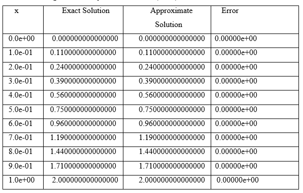

Fig 3.29 Comparison of Approximate and Exact Solutions of Eq. (3.206) for n=3.
Example 3.35 Consider the linear Fredholm integral equation [2]
![]()
The exact solution of Eq. (3.215) is
![]()
According to the proposed technique, consider the trail solution
![]()
Consider 5th order Bessel Polynomials, i.e. for n=5, we have Eq. (3.217) is

Substituting Eq. (3.218) into Eq. (3.215)

Now multiply Eq. (3.219) by ![]() j=,1,2,3,4,5 and integrating both side from 0 to π/4, we have
j=,1,2,3,4,5 and integrating both side from 0 to π/4, we have

The matrix form of Eq. (3.220) is

After solving we get,

Consequently we have the approximate solution is
![]()
Table 3.30 Comparison of the Exact Solution and Approximate Solutions of Eq. (3.215) for n=5, obtained using Bessel Polynomial Method

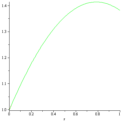
Fig 3.30 Comparison of Exact and Approximate Solutions of Eq. (3.215) for n=5.
Consider 10th order Bessel Polynomials, i.e. for we have Eq. (3.217) is


Substituting Eq. (3.221) into Eq. (3.215)
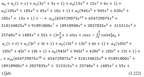
Now multiply Eq. (3.222) by ![]() j=0,1,2,…,10 and integrating both side from 0 to π/4, we have
j=0,1,2,…,10 and integrating both side from 0 to π/4, we have

The matrix form of Eq. (3.223) is
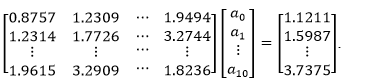
After solving we get
![]()
Consequently we have the exact solution is
![]()

Fig 3.31 Comparison of Exact and Approximate Solutions of Eq. (3.215) for n=10.
Table 3.31 Comparison of the Exact Solution and Approximate Solutions of Eq. (2.215) for using Bessel Polynomial Method

Consider 20th order Bessel Polynomials, i.e. for we have Eq. (3.217) is

Substituting Eq. (3.224) into Eq. (3.215)

Now multiply Eq. (3.225) by ![]() j=0,1,2,3,…,20. and integrating both side from 0 to π/4, we have
j=0,1,2,3,…,20. and integrating both side from 0 to π/4, we have


The matrix form of Eq.(3.226) is

After solving we get
![]()
Consequently we have the exact solution is
![]()
Table 3.32 Comparison of the Exact Solution and Approximate Solutions of Eq. (3.215) for n= 20, using Bessel Polynomial Method


Fig 3.32 Comparison of Approximate and Exact Solutions of Eq. (3.215) for n=20.
Example 3.36 Consider the linear Fredholm integral equation [2]
![]()
The exact solution of Eq. (3.227) is
![]()
According to the proposed technique, consider the trail solution
![]()
Consider 2nd order Bessel Polynomials, i.e. for n=2, we have Eq. (3.229) is

Substituting Eq. (3.230) into Eq. (3.227)

Now multiply Eq. (3.231) by ![]() j=0,1,2 and integrating both side from 0 to 1, we have
j=0,1,2 and integrating both side from 0 to 1, we have
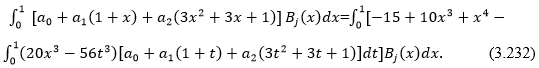
The matrix form of Eq. (3.232) is

After solving we get,
![]()
Consequently we have the approximate solution is
![]()
Table 3.33 Comparison of Exact and Approximate Solutions of Eq. (3.227), for obtained from Bessel Polynomials Method


Fig 3.33 Comparison of Exact and Approximate Solutions of Eq. (3.227) for n=3.
Consider 4th order Bessel Polynomials, i.e. for n=4, we have Eq. (3.229) is

Substituting Eq. (3.233) into Eq. (3.227) an proceeding as before we have the matrix form of Eq. (3.233) is

After solving we get
![]()
consequently we have the exact solution is
![]()
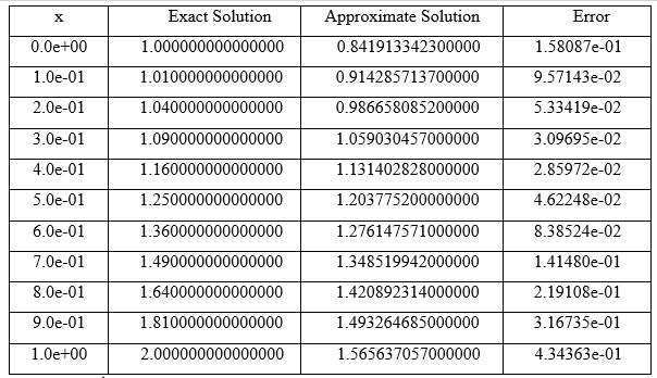
Example 3.37 Consider the weakly singular integral equation [2]
![]()
The exact solution of Eq. (3.234)
![]()
According to the proposed technique, consider the trail solution
![]()
Consider 1st order Bessel Polynomials, i.e. for n=1,we have Eq. (3.234) is

Substituting Eq. (3.236) into Eq. (3.234)
![]()
Now multiply Eq. (3.237) by ![]() j=0,1 and integrating both side from 0 to 1, we have
j=0,1 and integrating both side from 0 to 1, we have

the matrix form of Eq. (3.238) is

After solving we get ![]() Consequently we have the approximate solution is
Consequently we have the approximate solution is
![]()

Fig 3.34 Comparison of Exact and Approximate Solutions of Eq. (3.234) for n=1.
Table 3.34 Comparison of the Exact Solution and Approximate Solutions of Eq. (3.234) for using Bessel Polynomials Method
Consider 2nd order Bessel Polynomials, i.e. for n=2, we have Eq. (3.236) is

Substituting Eq. (3.239) into Eq. (3.234)
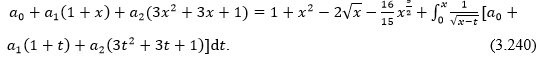
Now multiply Eq. (3.240) by ![]() j=0,1,2 and integrating both side from 0 to 1,we have
j=0,1,2 and integrating both side from 0 to 1,we have

the matrix form of Eq. (3.241) is

After solving we get ![]() and Consequently we have the exact solution is
and Consequently we have the exact solution is
![]()
Table 3.35 Comparison of the Exact Solution and Approximate Solutions of Eq. (3.234) for using Bessel Polynomials Method


Fig 3.35Comparison of Approximate and Exact Solutions of Eq. (3.234) for n=3.
References
[1] H.L. Krall and Orrin Frink, A new class of orthogonal polynomials: The Bessel polynomials, Trans. Amer. Math. Soc.65 (1949), 110-115.
[2] A.M.Wazwaz, Linear & Nonlinear Integral Equations Method and Applications, Springer Heidelberg Dordrecht London, New York, 2011.